Exploring methods to create a multivariate t-distributed random matrix

This document is part of the the mvrt package. See the README.md for more information on download and installation.

Objective

The objective of this R package vignette is to investigate the various ways of creating multivariate normal/t distributions. An algorithm using Cholesky decomposition is used; first in R code, then in C++ code. This is compared to existing methods for creating multivariate random matrices, such as MASS::mvrnorm and mvtnorm::rmvt.

The matrices are compared using summary statistics and graphics (histograms). The distributions are assessed for “believability”. Methods are also explored for ensuring that the specified correlation/covariance structure is preserved, despite the random process of number generation. Finally, benchmarking is perfromed to determine performance differences.

Setup

Defining the data

We will specify the sample n pairs, means, correlation matrix, and variances. The correlation matrix and variances will be used to generate a covariance matrix, which will be used by the random number generator.

n <- 30
mu <- c(5,4)
R <- matrix(c(1,.9,.9,1),2,2)
var <- c(2.5,2)

S <- mvrt::convert_R2S(R, var)

Defining the multivariate t-distributed random matrix generator functions

First we will define the random number generator functions in R. We will compare the performance of R code with- and without for loops. Well-optimized R code may be sufficiently performant as to not warrant the implementation of a compiled alternative.

# With a for loop
mvrt_R_a <- function(n, mu, S, df = n - 1) {

  g.t <- t(chol(S))

  bivMat <- matrix(0,nrow = length(mu), ncol = n)

  for (i in seq_len(n)) {
    bivMat[,i] <- mu + g.t %*% rt(length(mu), df)
  }

  t(bivMat)

}

# Without a for loop
mvrt_R_b <- function(n, mu, S, df = n - 1) {
  
  g <- chol(S)
  
  random_matrix <- matrix(rt(n*length(mu), df),nrow = length(mu))
  deviation <- t(g) %*% random_matrix
  
  t(mu + deviation)
  
}

Compiling and loading the C++ mvrt random matrix generator

Next we will load in a function written in C++. The expectation is that the C++ code will be faster than the R code, possibly by several orders of magnitude.

Rcpp::sourceCpp("../src/mvrt.cpp")

The code that was loaded is below.

#include <RcppArmadillo.h>
// [[Rcpp::depends(RcppArmadillo)]]

using namespace Rcpp;

//' @rdname mvrt
//' @export
// [[Rcpp::export]]
arma::mat mvrt(int n, arma::vec mu, arma::mat S, int df=1)
{

  // Cholesky decomp and transpose covariance matrix
  arma::mat g = chol(S).t();

  // Generate the random data
  auto x_vec = rt(mu.size() * n, df);
  arma::mat x = arma::mat(&x_vec[0], mu.size(), n, false, true);

  // Give the random data covariance structure and add mean offset
  x = g * x;
  x.each_col() += mu;

  return x.t();
}

Define our function for getting a distribution of correlation coefficients

This function will take a function and its arguments and run it a specified number of times, performing a correlation on the output and extracting the off-diagonal element. Essentially, we can use this to run each random number generator an arbitrary number of times and get the Pearson’s correlation for each pair of vectors created. This can be used to examine the distribution of correlation coefficients that can be expected from the random generation processes. Note the random seed parameter which can be set for reproducibility.

get_cor_dist <- function(FUN, times, ..., seed = 999) {
  
  set.seed(seed)
  
  FUN <- match.fun(FUN)
  
  my_call <- as.call(list(FUN, ...))
  
  out <- numeric(times)
  
  for (i in seq_len(times)) {
    
    out[i] <- cor(eval(my_call))[2]
    
  }
  
  out
  
}

Generating the distributions of correlation coeffiencts using sever random matrix generators

Using the function above, we will create similar multivariate t-distributed (or normally-distributed) random matrices using several functions.

mvrtRa_dist <-  get_cor_dist(mvrt_R_a, 100, n, mu, S)
mvrtRb_dist <-  get_cor_dist(mvrt_R_b, 100, n, mu, S)
mvrt_dist <-    get_cor_dist(mvrt, 100, n, mu, S, n - 1)  
MASS_dist <-    get_cor_dist(MASS::mvrnorm, 100, n, mu, S)
mvtnorm_dist <- get_cor_dist(mvtnorm::rmvt, 100, n, S, n - 1)

Analysis

Checking the algorithm

Homogenous outputs

First let’s check that our three home-grown functions produce identical results.

if (identical(mvrtRa_dist, mvrt_dist) && identical(mvrtRb_dist, mvrt_dist)) {
  message("Distributions of correlation coefficients are identical")
} else {
  message("Distributions of correlation coefficients are NOT identical")
}

## Distributions of correlation coefficients are NOT identical

if (
  identical(
    (mvrt_sample <- {set.seed(999); mvrt(n, mu, S, n - 1)}),
    {set.seed(999); mvrt_R_a(n, mu, S)}
    ) &&
  identical(
    mvrt_sample,
    {set.seed(999); mvrt_R_b(n, mu, S)}
    )
) {
  message("Random samples generated match")
} else {
  message("Random samples generated do NOT match")
}

## Random samples generated do NOT match

It appears that we are successful in that the three functions produce identical output. Therefore, we must only examine one function’s output when doing distribution analysis, rather than all three.

Inspecting outputted means and variances

Let’s run a couple of checks to make sure that the algorithm is at least giving us data with approximately correct means and variances.

# Mean mu
colMeans(t(sapply(lapply(rep(30,100), mvrt, mu, S, n - 1),colMeans)))

## [1] 4.943320 3.951612

# Mean var
colMeans(t(sapply(lapply(rep(30,100), mvrt, mu, S, n - 1), apply, 2, var)))

## [1] 2.607499 2.103790

Means are close and variances are just a little higher than those specified in the covariance matrix, which we might expect from a relatively small sample size.

An individual sample

Let’s pull a single sample of n = 30. We can check the mean, variance, and correlation.

mvrt_sample <- mvrt(n, mu, S, n - 1)

colMeans(mvrt_sample)

## [1] 5.261327 4.106697

apply(mvrt_sample, 2,var)

## [1] 2.157964 1.204207

cor(mvrt_sample)

##           [,1]      [,2]
## [1,] 1.0000000 0.8381404
## [2,] 0.8381404 1.0000000

How does a plot of the data look?

plot(mvrt_sample)
# Regression line
abline(lm(mvrt_sample[,2] ~ mvrt_sample[,1]), col = "red")

# Center of points
points(mean(mvrt_sample[,1]), mean(mvrt_sample[,2]), col = "blue", pch = 22)

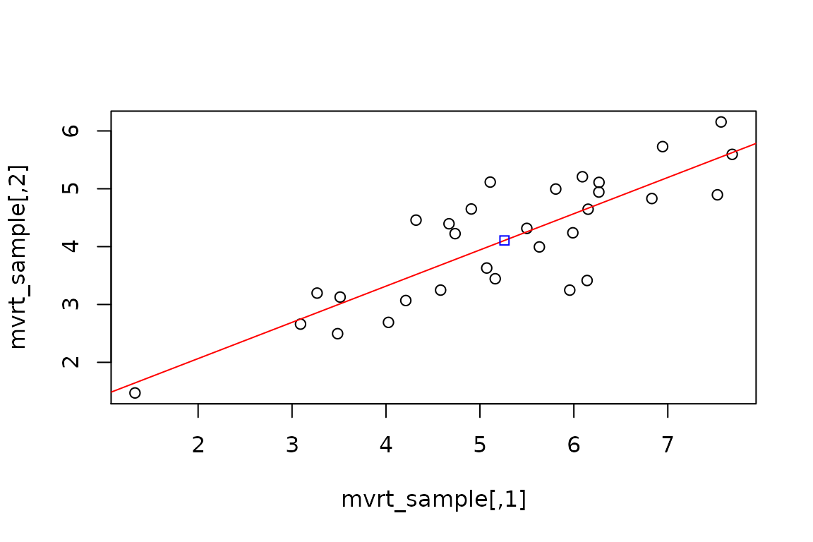
OK. So we are fairly confident that we are getting the data we requested. Now let’s look at how the correlation coefficients are distributed over several simulations.

Comparing the correlation coefficient distributions of the various functions

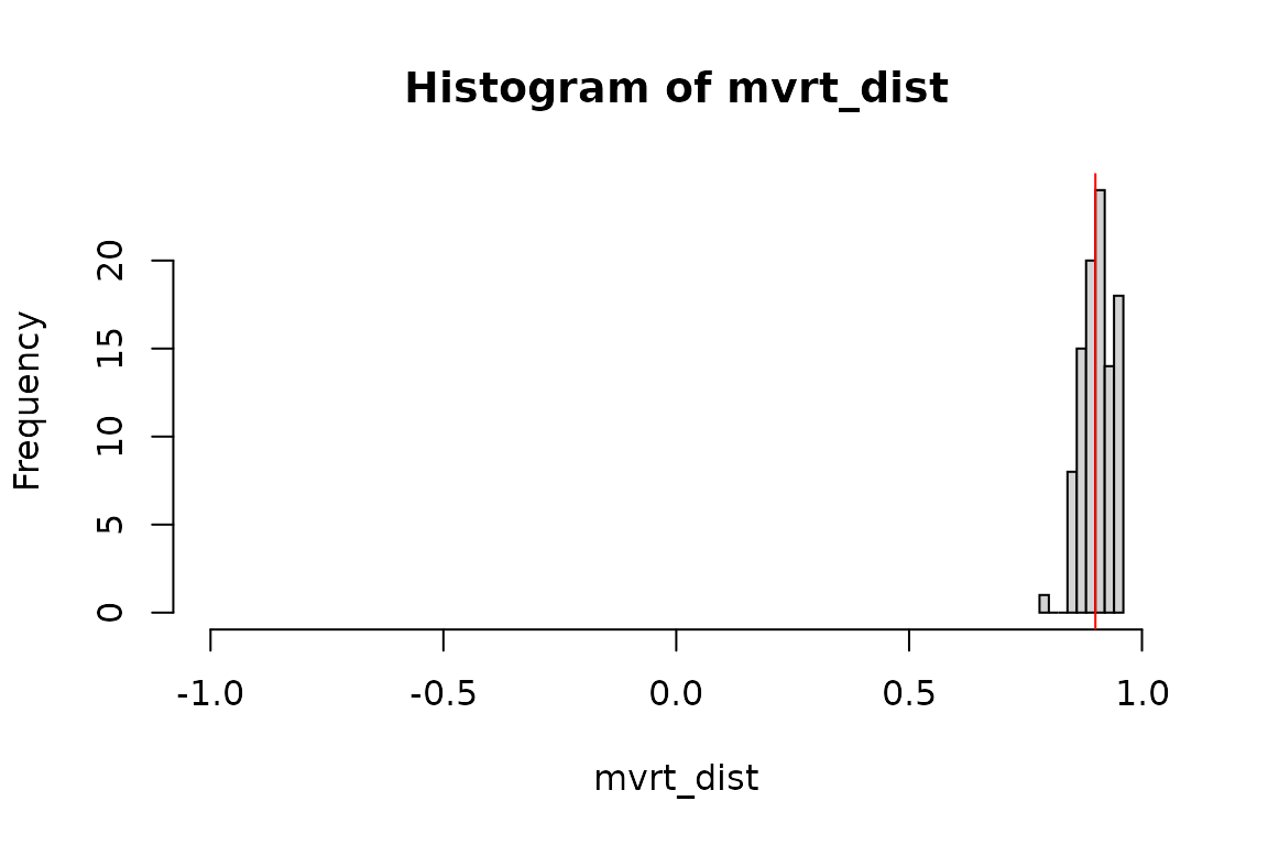
# Summary of the distributions
summary(mvrt_dist)

##    Min. 1st Qu.  Median    Mean 3rd Qu.    Max.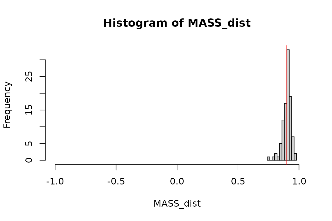 
##  0.7809  0.8804  0.9084  0.9043  0.9316  0.9588

summary(MASS_dist)

##    Min. 1st Qu.  Median    Mean 3rd Qu.    Max.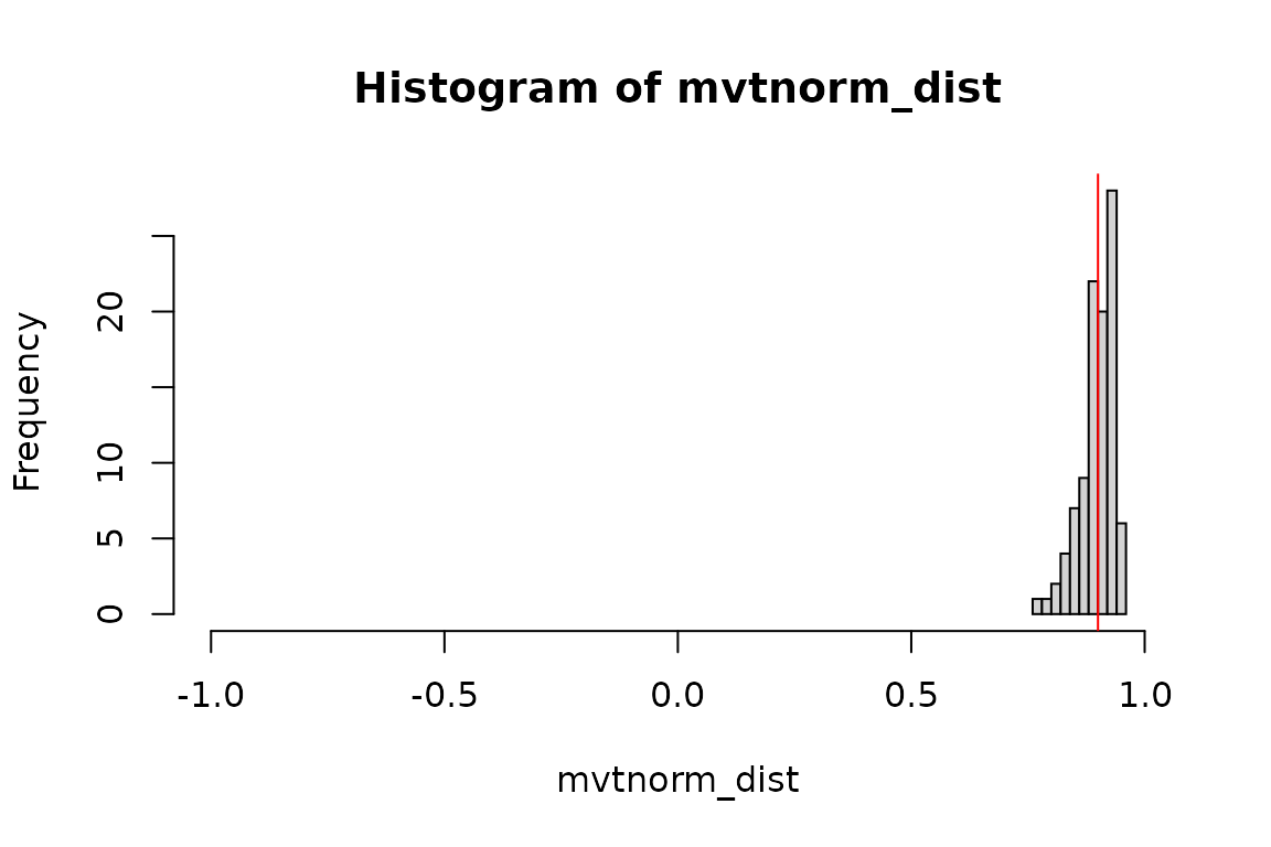 
##  0.7500  0.8831  0.9082  0.9010  0.9219  0.9661

summary(mvtnorm_dist)

##    Min. 1st Qu.  Median    Mean 3rd Qu.    Max. 
##  0.7777  0.8816  0.9030  0.8980  0.9251  0.9570

# Graphical representations
my_hist <- function (data) {
  hist(
    data, 
    xlim = c(-1,1), 
    breaks = "fd", 
    main = paste("Histogram of",deparse(substitute(data))),
    xlab = deparse(substitute(data))
  )
  
  abline(v = 0.9, col = 'red')
}

my_hist(mvrt_dist)

my_hist(MASS_dist)

my_hist(mvtnorm_dist)

Guaranteeing outputs are within a specified range

What if we would like to specify that the matrix of values returned is within a reasonable margin to the specified correlation coefficient? This can be done through iterative generation of the random sample with acceptance checks at each step. A matrix norm of the difference in correlation matrices (between generated and specified) may be used as an intuitive check. We may specify that the maximum modulus of the difference between specified and returned correlation matrix elements is below a given threshold.

The determinant may also be used (and is potentially faster). However the norm may be more easily interpreted since the element-wise maximum modulus is a good way for the user to specify an acceptance criterion.

Choosing the matrix norm over the determinant

Why use the matrix norm rather than the determinant or some other measure? Because it is the most intuitive. The matrix norm is computed several ways. We will use the maximum modulus (absolute value) method, which is equivalent to performing max(abs()) on a matrix. This means that in we can specify the maximum devation of any element within the resultant correlation matrix generated by random sample versus the specified. For example, specifying a maximum matrix norm of 0.05 means that the Pearson’s correlation generated from outputted values will be within \(\pm\) 0.05 of the Pearson’s correlation used as the input correlation matrix (as derived form the input covariance matrix).

To demonstrate, we will create a reference correlation matrix and then compare it to a set of contender matrices using the determinant and norm.

# A single reference matrix
R_ref <- mvrt::make_cor_mat(.9)
R_ref

##      [,1] [,2]
## [1,]  1.0  0.9
## [2,]  0.9  1.0

# A set of test matrices
R_test <- lapply(seq(.5,1,.05), mvrt::make_cor_mat)
R_test[[1]]

##      [,1] [,2]
## [1,]  1.0  0.5
## [2,]  0.5  1.0

# What does the determinant look like for the difference matrices?
sapply(R_test, function(a,b) det(a - b), R_ref)

##  [1] -0.1600 -0.1225 -0.0900 -0.0625 -0.0400 -0.0225 -0.0100 -0.0025  0.0000
## [10] -0.0025 -0.0100

# And the matrix norm?
sapply(R_test, function(a,b) norm(a - b, "m"), R_ref)

##  [1] 0.40 0.35 0.30 0.25 0.20 0.15 0.10 0.05 0.00 0.05 0.10

The user is more likely to understand how to specify a max norm than a max determinant.

Iterative function definitions

Below we see two function definitions which perform the same task but implement different programming techniques. The first utilizes recursive function calls, while the second uses a for loop to repeat sample generation until the acceptance criterion is met.

# Using recursive function calls
mvrt_R_c <- function(n, mu, S, df = n - 1, max.norm = 0.05, type.norm = "m") {
 
  g <- chol(S)
 
  random_matrix <- matrix(rt(n*length(mu), df),nrow = length(mu))
  deviation <- t(g) %*% random_matrix
 
  out <- t(mu + deviation)
 
  if (norm(cov2cor(S) - cor(out), type = type.norm) <= max.norm) {
    return(out)
  } else {
    eval(match.call())
  }
 
}


# Using the for loop
mvrt_R_d <- function(
  n,
  mu,
  S,
  df = n - 1,
  max_norm = 0.05,
  max_iterations = 1000,
  type_norm = "m")
{

  g.t <- t(chol(S))

  R_ref <- cov2cor(S)

  for (iterations in seq_len(max_iterations)) {

    random_matrix <- matrix(rt(n*length(mu), df),nrow = length(mu))
    deviation <- g.t %*% random_matrix

    if (norm(R_ref - cor(t(mu + deviation)), type = type_norm) <= max_norm)
      return(t(mu + deviation))

  }

  stop(
    "Correlation structure with max norm of ", max_norm,
    " was not obtained in ", max_iterations, " iterations"
    )

}

We may also include a C++ function to achieve this.

Rcpp::sourceCpp("../src/mvrt2.cpp")

The code that was loaded is below.

#include <RcppArmadillo.h>
// [[Rcpp::depends(RcppArmadillo)]]

using namespace Rcpp;

//' @rdname mvrt
//' @export
// [[Rcpp::export]]
arma::mat mvrt2(
    int n,
    arma::vec mu,
    arma::mat S,
    int df=1,
    double max_norm=2,
    int max_iterations=1000
  )
{

  // Cholesky decomp and transpose covariance matrix
  arma::mat g = chol(S).t();

  // Get correlation matrix of user-input S matrix
  arma::mat V_sqrt_inv = diagmat(1 / sqrt(S.diag()));
  arma::mat target_cor = V_sqrt_inv * S * V_sqrt_inv;

  for (int iteration=0; iteration < max_iterations; iteration++) {

    // Generate the random data
    auto x_vec = rt(mu.size() * n, df);
    arma::mat x = arma::mat(&x_vec[0], mu.size(), n, false, true);

    // Give the random data covariance structure and add mean offset
    x = g * x;
    x.each_col() += mu;

    // Compare to target and retrun if meets specification
    arma::mat diff_matrix = abs(cor(x.t()) - target_cor);

    if (diff_matrix.max() <= max_norm)
      return x.t();
  }

  stop(
    "Did not generate matrix with max norm of %f in %i iterations",
    max_norm,
    max_iterations
  );

}

Checking our work

Now lets see if the distributions tighten up with our new functions. We should now see that the correlation coefficient of each of our randomly generated samples will not stray more than 0.05 from the correlation of the correlation matrix used to specify the covariance structure of the data.

mvrtRc_dist <-  get_cor_dist(mvrt_R_c, 100, n, mu, S)
mvrtRd_dist <-  get_cor_dist(mvrt_R_d, 100, n, mu, S)
mvrt2_dist <-   get_cor_dist(mvrt2,    100, n, mu, S, n - 1, 0.05)

if (identical(mvrtRc_dist, mvrtRd_dist) && identical(mvrtRc_dist, mvrt2_dist)) {
  message("Distributions of correlation coefficients are identical")
} else {
  message("Distributions of correlation coefficients are NOT identical")
}

## Distributions of correlation coefficients are identical

summary(mvrtRc_dist)

##    Min. 1st Qu.  Median    Mean 3rd Qu.    Max. 
##  0.8545  0.8801  0.9070  0.9028  0.9257  0.9472

my_hist(mvrtRc_dist)

This appears to have worked. Compare with distributions explored in the previous section.

We can also specify a different covariance structure and check again. This demonstrates the usage of the various function definitions we have created for this exercise.

summary(
  get_cor_dist(
    mvrt_R_d, 
    100, 
    n, 
    mu, 
    mvrt::convert_R2S(mvrt::make_cor_mat(0.2),var)
    )
  )

##    Min. 1st Qu.  Median    Mean 3rd Qu.    Max. 
##  0.1502  0.1727  0.2059  0.2012  0.2254  0.2500

Not surprisingly, the correlation coefficients remain within [0.15,0.25].

Benchmarking

Let’s see how the functions compare in speed.

microbenchmark::microbenchmark(
  # No data checks
  mvrt_R_a(n, mu, S),               # 'for' loop
  mvrt_R_b(n, mu, S),               # Optimized R code
  mvrt(n, mu, S, n - 1),            # C++ code
  
  # Iterative checking
  mvrt_R_c(n, mu, S),               # Recursive call
  mvrt_R_d(n, mu, S),               # 'for' loop
  mvrt2(n, mu, S, n - 1, 0.05),     # C++ code
  
  # Available packages on CRAN
  MASS::mvrnorm(n, mu, S),
  mvtnorm::rmvt(n, S, n - 1) + mu
)

## Unit: microseconds
##                             expr     min       lq      mean   median       uq
##               mvrt_R_a(n, mu, S)  90.661 108.4645 121.40708 116.6335 124.3230
##               mvrt_R_b(n, mu, S)  20.899  25.0180  30.97702  27.5790  32.1935
##            mvrt(n, mu, S, n - 1)   8.147  11.3415  14.22796  12.7420  14.0440
##               mvrt_R_c(n, mu, S)  47.564  58.7980  87.52966  65.3965  92.3645
##               mvrt_R_d(n, mu, S)  55.022  64.5345  79.60625  72.3330  86.4830
##     mvrt2(n, mu, S, n - 1, 0.05)   9.584  13.9980  19.26501  15.2845  20.9425
##          MASS::mvrnorm(n, mu, S)  57.528  69.0395  77.12211  72.7785  80.7545
##  mvtnorm::rmvt(n, S, n - 1) + mu 222.389 242.6085 264.10592 250.9265 266.4525
##      max neval
##  210.871   100
##   81.664   100
##   36.124   100
##  389.618   100
##  179.257   100
##   90.935   100
##  177.896   100
##  489.337   100

I know the :: operator has a performance cost for those CRAN packages. It may be interesting to try the benchmarking with loaded packages, too.

MASS_mvrnorm <- MASS::mvrnorm
mvtnorm_rmvt <- mvtnorm::rmvt

microbenchmark::microbenchmark(
  MASS::mvrnorm(n, mu, S),
  MASS_mvrnorm(n, mu, S),
  mvtnorm::rmvt(n, S, n - 1) + mu,
  mvtnorm_rmvt(n, S, n - 1) + mu
)

## Unit: microseconds
##                             expr     min       lq      mean   median      uq
##          MASS::mvrnorm(n, mu, S)  52.782  59.6945  67.07632  64.7465  69.097
##           MASS_mvrnorm(n, mu, S)  45.846  52.4620  60.08722  57.8490  60.704
##  mvtnorm::rmvt(n, S, n - 1) + mu 212.948 222.8000 252.81270 230.5440 244.164
##   mvtnorm_rmvt(n, S, n - 1) + mu 202.570 214.8225 230.15693 220.5860 236.567
##       max neval
##   140.642   100
##   152.106   100
##  1619.700   100
##   435.766   100

Conclusion

Clearly, rolling your own C++ code is superior. But given the performance gain from removing the for loop from our original R function, optimization of R code cannot be underestimated. Given that the well-written R code is comparably performant within an order of magnitude, the switch to C++ is likely not worth the additional effort in this case.

Paul W. Egeler, MS, GStat

2020-10-06